1) Computational Research on Alloy Design and Plastic Flow Behavior of TRIP Steels coupled with Estimation of the Model Parameters by Bayesian Approach
Transformation-Induced Plasticity (TRIP) Steels are a group of low-alloy steels which can provide an appropriate combination of strength and fracture toughness due to high strain hardening arising from strain-induced martensitic transformation (SIMT) during plastic deformation. These interesting properties make these high strength steels desirable for automotive industry by offering lower weight and higher safety for vehicles. TRIP steels are characterized by their multi-phase microstructure, which includes ferrite, bainite, retained austenite, and martensite. Retained austenite as a dispersed phase in ferritic matrix plays an important role to obtain high strain hardening in this group of steel. In this regard, it has been found that the main characteristics of this phase are its grain size, carbon concentration, and volume fraction.

Fig. 1
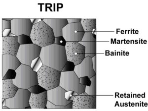
Fig. 2
Our studies about TRIP steels can be categorized in three different areas:
- Heat treatment design
- Modelling of plastic flow behavior
- Bayesian parameter calibration of the plastic flow model
– Heat Treatment Design:
It was indicated that the austenite can be retained in the microstructure at room temperature using a two-step heat treatment, including intercritical α+𝛾 annealing (IA) and bainitic isothermal transformation (BIT). As shown in Fig. 3, different stages of heat treatment lead to the formation of various phases in the final microstructure. This process can be observed in the diagram of temperature in terms of austenite carbon content in Fig. 4.
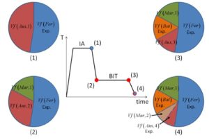
Fig. 3
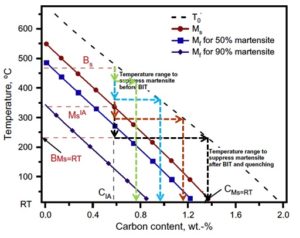
Fig. 4
However, we applied Thermo-Calc software to change the common two-step processing to three steps for Fe-0.32C-1.56Si-1.42Mn alloy (Fig. 5 and 6) in order to suppress the formation of martensite during heat treatment, which is detrimental for mechanical properties. According to our predictions, this processing results in the formation of about 22% austenite, which can considerably improve the mechanical properties of the given alloy.
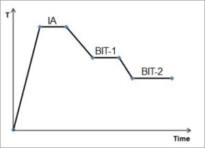
Fig. 5
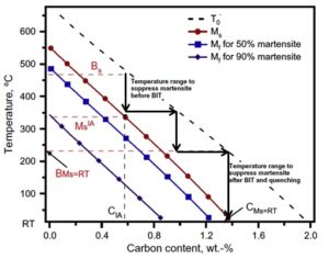
Fig. 6
– Modelling of plastic flow behavior:
In this model, Shear stress for each microstructural phase is defined in terms of the contribution of different hardening mechanisms, including the Peierls force, solid solution strengthening, long-range back stress, dislocation strengthening, and precipitation strengthening. Rivera model [Modeling Simul. Mater. Sci. Eng. 22:015009,2014] based on a thermos-statistical theory of plasticity has been used in this research to predict dislocation density evolution (dislocation hardening mechanism) of TRIP steels during plastic deformation. In fact, this model has been applied for each phase in the microstructure, and the plastic flow behavior is subsequently estimated using an iso-work approximation approach. The deformation-induced martensitic transformation has been also modeled based on Haidemenopoulos theoretical method [Mter. Sci. Eng. A 615:416-23,2014].
– Bayesian parameter calibration of the plastic flow model:
Estimation of model parameters is a fundamental matter in science and engineering, which is usually overlooked by engineers. The advent of high-speed computers causes more attention to Bayesian approach for the analysis of model parameters, particularly those are based on Markov chain Monte Carlo (MCMC) methods. It has been illustrated that MCMC-based Bayesian approaches can result in better parameter calibrations for multi-level models compared to other likelihood based techniques. Therefore, we have applied MCMC-Standard Metropolis-Hastings algorithm to calibrate the sensitive parameters in the plastic flow model through sampling from an adaptive proposal distribution for posterior probability density function of parameters. In this approach, the model is trained with different experimental data sequentially or simultaneously to estimate parameters and their uncertainties. The initial prior probability distributions of parameters and likelihood functions are determined from the data in literature. Metropolis-Hastings ratio is used as a criterion for acceptance/rejection of randomly selected samples in order to generate a number of samples which can represent the posterior probability distribution of parameters. These distributions are utilized for the determination of prior distributions for next data training in the case of sequential data trainings. The details of our methodology can be observed in Fig. 7. The calibrated parameters and their uncertainties are also shown in Table 1. For plotting strain-stress curves and their uncertainties after the calibrations, the concept of “propagation of error” has been used to propagate the uncertainty of parameters obtained from the posterior distributions to the overall error of the model, i.e., the uncertainty of stress at any given strain. Stress-strain curves and their uncertainty bands after sequential and simultaneous calibration have been demonstrated for all experimental conditions in Fig. 8(a) and (b). The black lines correspond to the plausible mean parameter values obtained after calibrations, and the blue and (blue + green) shaded areas are related to 68% and 95% Bayesian confidence intervals of the model predictions, respectively.
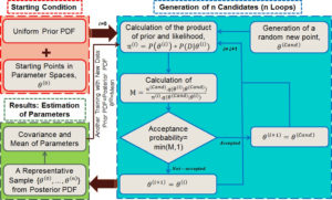
Fig. 7
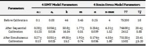
Table 1
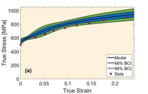
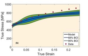
Fig. 8 (a-b)
2) Bayesian Calibration of the Precipitation Model implemented in MatCalc
The first step for solving optimization (reverse) problem from performance to composition and processing is the calibration of the physical rigorous models that are used for optimal experimental design and subsequent model refinement. Precipitation model is one of these models, which connects chemistry and processing to micro-mechanical model. While NiTiHf thermodynamics database has been developing by experiments and ThermoCalc optimizations, we decided to develop and calibrate NiTi binary precipitation model by the existing NiTi database. This can facilitate the implementation and calibration of ternary precipitation model in the next step of project.
The most sensitive parameters for calibration have been recognized using model forward analysis, which are matrix/precipitate interfacial energy, diffusion correction, nucleation site density, nucleation constant, and shape factor (D-disk diameter/h-disk height). Markov Chain Monte Carlo (MCMC)-Metropolis Hasting Algorithm has been applied for the parameter calibrations. In this approach, prior knowledge including the initial values of parameters and their range obtained from literature or MatCalc© default in addition to experimental data are fed to Matlab MCMC toolbox. In this regard, non-informative (e.g., uniform) probability density functions (PDFs) can be considered as parameter prior distributions since no statistical information has been found for the given model parameters, and 9 experimental data has been extracted from Panchenko’s work. In MCMC toolbox, n samples of parameter vector are generated by random walk. It should be noted that there is a vector of model outputs with three elements, including Ni content of matrix, volume fraction of precipitates, and mean precipitate size, which can simultaneously be compared with its corresponding vector of experimental results in order to calibrate the above-mentioned parameters. At the end of this process, these parameter samples indicate the posterior PDFs of given parameters whose mean and covariance would be parameter optimal values and uncertainties, respectively. These calibrated parameters and their uncertainties are utilized to determine the uncertainty of model outputs using propagation of uncertainty:
Forward analysis of NiTi precipitation model showed there may be a relationship between matrix/precipitate interfacial energy and two of the model inputs, i.e., aging temperature and Ni nominal composition. For this reason, we decided to calibrate the above mentioned model parameters with each experimental data individually to find the optimum value for the interfacial energy in each experimental case. The other sensitive parameters have also been involved in calibration to consider their possible correlation with the interfacial energy. As an example, one of these calibrations is explained as follows.
After MCMC sampling, the correlation between each two parameters have been plotted to see how the change in one of them can affect the other one in optimal parameter space. One of these plots has been shown in Fig. 9a. The regions with high density of sample points (such as the red region in this figure) indicate the convergence of parameters to their optimum values. According to Fig. 9b, the posterior PDF of interfacial energy shows two picks. It seems that the peak demonstrated with blue arrow contains the optimum value for this parameter, and red arrow probably indicates a fake peak since it is around the initial value chosen for this parameter. In this case, it can result from the disability of MCMC technique to escape the local trap in the beginning of sampling. In order to find the transition point to the optimal peak, cumulative mean of samples has been plotted as observed in Fig. 9c. After around 8000 sampling points for interfacial energy, there is a sudden change in the plot trend which can correspond to this transition, Therefore, the first 8000 generations has been considered as burn-in period (left side of red dotted line) and removed for the calculation of optimum values for parameters and their uncertainties. Fig. 9d verifies that the fake peak would be eliminated after removal of the first 8000 generations. In table 2 and 3, the calibrated parameters and their corresponding model outputs with the uncertainties have been listed just for one calibration. Table 2 indicates a very good agreement between model results and experimental data.
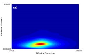
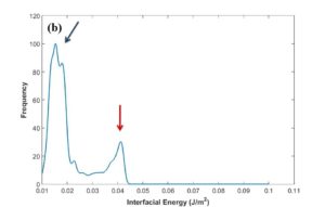
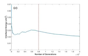
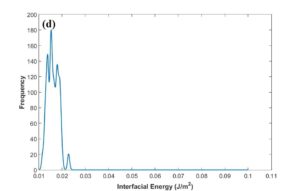
Fig. 9 (a-d)

Table 2

Table 3
If the interfacial energy values obtained from the model calibration with each one of experiments are plotted in terms of aging temperature and nominal Ni content, a polynomial surface can be fitted as shown in Fig. 10. After inserting the fitted surface equation in the model, we have calibrated the other four model parameters with all nine experimental data together, based on the same approach mentioned above. The results for calibrated parameters and the model outputs corresponding to each experimental case have been reported in table 4 and 5, respectively. Although the model results do not fit the data exactly, most of the data is located in 95% Bayesian confidence intervals of the model results.
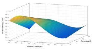
Fig. 10

Table 4
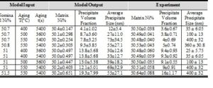
Table 5
It should be noted that the discrepancy function between the mean value of model results and experimental data (including natural uncertainty, missing physics, and data uncertainty) can be obtained through Gaussian process which can correct/improve our model. In addition, the co-kriging approach is going to be used in order to take advantage of physical model and surrogate model at the same time by finding the correlation of these two models in the design space.
3) Parameter Calibration in Phase Field Modeling
Phase field modelling is one of the most powerful approaches for the simulation of microstructural changes in materials; however, the model calibration and uncertainty quantification is a very hard task through conventional deterministic and probabilistic techniques due to high computational cost. Therefore, different global optimization approaches can be used to tackle the issue of calibration in these models such as Bayesian Global Optimizations (BGO), Knowledge-Gradient Optimizations (KGO), Efficient Global Optimizations (EGO), etc.
The phase field model parameters will be calibrated against two inter-metallic layer thicknesses. In order to not struggle with high multi-dimensionality in this work, the most sensitive parameters are found through a forward model analysis approach. In this sensitivity analysis, a two-level fractural factorial design has been considered to generate a fractional combination of model parameters for forward analysis which is an efficient technique for taking parameter interactions into account. Then, the analysis of variance (ANOVA) is also applied to rank the importance of parameters based on the p-values.
the corresponding multidimensional parameter space will be exploited and explored using EGO method in order to minimize the objective errors between the experimental data and model results; The objective error is the cumulative difference between all the available experimental time points and their corresponding model results for both thicknesses at each processing temperature. Therefore, just one scalar value is calculated for cumulative error which is minimized to find the optimum values for model parameters. This means a single objective optimization problem in this work. In this regard, there is a need for a surrogate model on parameter space with associated confidence intervals. For this purpose, a surrogate model based on Gaussian Process (GP) is built on some random points in the parameter space, which are generated by the Latin Hypercube Sampling (LHS) approach.
At the end, the expected improvement is calculated based on the surrogate function all over the parameter space. The parameter values associated with the maximum expected improvement is used as the next point for forward analysis. This process continues till a stopping criteria is satisfied.
